Published · Oct. 2025
Positivity bounds in scalar-QED EFT at one-loop level
One-loop scattering amplitudes and dispersion relations reveal when tree-level positivity bounds survive quantum corrections in scalar-QED EFT.
Yunxiao Ye, Xiao Cao, Yu-Hang Wu, and Jiayin Gu
Journal of High Energy Physics 10 (2025) 084 · Published 10 October 2025
Journal article · arXiv:2507.06302 · Full paper (PDF)
Selected passages and original figures from our paper. Section headings and brief transitions have been adapted for this page; figure and equation numbers refer to the published article.
Motivation
Effective Field Theory (EFT) is a powerful framework that connects physics at different scales. In an EFT, the effects of the underlying ultraviolet (UV) physics can be parameterized as a series of higher dimensional operators in the low-energy effective Lagrangian, suppressed by the cutoff scale Λ.
If the underlying physics is unknown, the Wilson coefficients should be regarded as free parameters to be determined by experiments. However, not all Wilson coefficients are free — unitarity, analyticity, and crossing symmetry of the S-matrix impose nontrivial constraints, requiring the Wilson coefficients of certain dimension-8 (dim-8) or even higher dimensional operators to be positive. This is commonly denoted as positivity bounds in an EFT.
Things are more complicated at the loop level, where logarithmic terms also enters the amplitudes. Furthermore, it is well known that even the definitions of renormalized parameters are ambiguous, which depends on the renormalization schemes and renormalization group (RG) running.
The implication of positivity bounds at the loop level are also of particular relevance for their experimental probes. For instance, a observation of the apparent violation of positivity bounds could merely be an indication that the tree-level assumption is false, rather than the break down of the fundamental principles of quantum field theory.
From dispersion relations to scalar-QED EFT
When the external particles include gauge bosons (spin-1 particles), the situation can be very different from the scalar case and requires careful studies, since gauge invariance puts stringent restrictions on the possible forms of couplings and amplitude structures. In particular, the gauge interactions come from kinetic terms, so they could not mix particles with different masses.
As a first step towards a more complete understanding of positivity bounds for gauge theories and the SM, in this paper we consider the simplest gauge theory — scalar QED and its EFT, and study the positivity bounds in this theory at the one-loop level.
We assume that the UV theory is a weakly coupled quantum field theory (QFT), so that the classification of loop orders is meaningful to begin with. We further assume all the particles in the UV theory — massless or massive — have spin less or equal to one.
We will focus on the elastic processes γϕ → γϕ and γγ → γγ, where the initial and final state photons (γ) have the same polarization, while two incoming photons can have different polarizations. In each process, we compute the relevant dispersion relation up to the dim-8 and one-loop levels.
The dispersion relation connects the forward elastic amplitude to a positive integral over total cross sections. The contour deformation underlying this relation is shown in Figure 1.
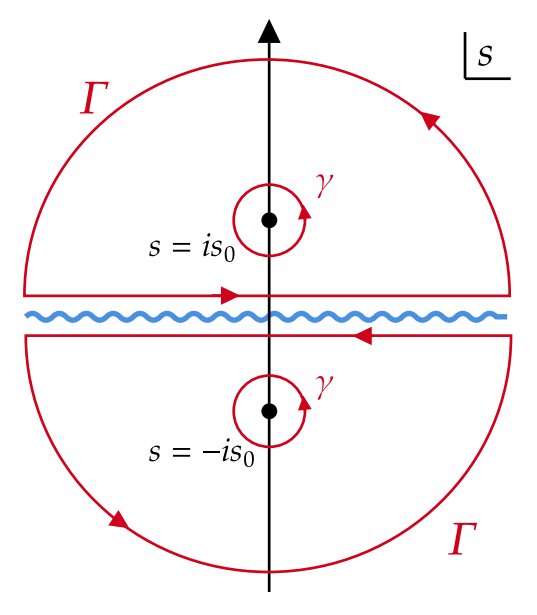
In particular, for polynomials of s, only the s2 (or even higher powers of s) term in the amplitude contributes to Σ, but with an extra factor of log(s) all terms could contribute. This means that the dim-4 and dim-6 one-loop contributions generally enters the dispersion relation.
Photon–scalar scattering
For γϕ → γϕ, the tree-level positivity bound is c(1)F²D²ϕ² ≤ 0. At one loop, the dispersion relation also receives contributions from four-scalar operators, illustrated in Figure 4.
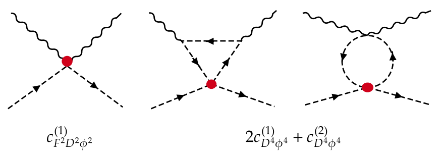
The potential IR divergences also require careful treatments. In particular, divergences of the form log(−t) are regulated with a small mass term when necessary, while IR poles of the form 1/ε are shown to be absent in the dispersion relation at the one-loop level in the UV theory.
With this regulator, the forward-limit bound takes the following form:

Again, here we assume the combination 2c(1)D⁴ϕ⁴ + c(2)D⁴ϕ⁴ is generated at the tree-level. Then, assuming μ2 is not too small (i.e. μ2 ≫ m2), the last term in eq. (4.14) is positive and could easily dominate over the first two terms. As such, eq. (4.14) no longer implies the tree-level bound c(1)F²D²ϕ² ≤ 0.
This means that, while c(1)F²D²ϕ² does not necessarily satisfy the tree-level bound c(1)F²D²ϕ² ≤ 0, its β-function always tend to restore the tree-level bound in the IR, so c(1)F²D²ϕ² ≤ 0 is always satisfied for sufficiently small μ (assuming the perturbation theory is still valid). However, it should be emphasized that by changing the value μ we do not obtain new positivity bounds — it merely changes the definition of couplings, and for small μ we are simply absorbing a large positively-bounded log term in the definition of c(1)F²D²ϕ².
The paper verifies these findings in two UV models with a heavy scalar extension (Section 4.2). If the four-scalar coefficients are also loop-generated, their contributions become sub-leading at the UV one-loop order: the tree-level bound remains valid, and the sign of the β-function cannot be determined from the dispersion relation at that order.
Photon–photon scattering
For γγ → γγ, on the other hand, all Wilson coefficients that contribute at the one-loop level are themselves generated at the one-loop level in the UV, so the one-loop contributions in the EFT are actually two-loop effects in the UV theory. In this case, the tree-level positivity bounds manifestly hold at the one-loop level in the UV theory.
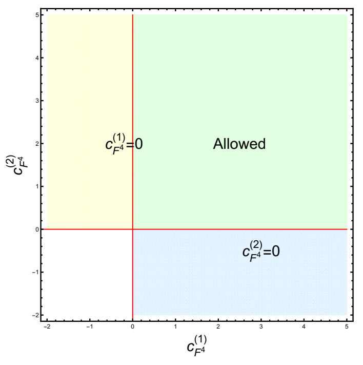
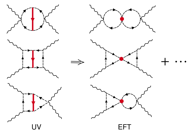
The dispersion relations provide a verification of these tree-level bounds. Extending the reasoning beyond one loop in the UV theory, however, requires additional contributions at the same UV loop order. Figure 6 illustrates a two-loop EFT contribution from a tree-level-generated four-scalar coefficient that must also be included.
Conclusion
In this paper, we derived the one-loop positivity bounds of the γϕ → γϕ and γγ → γγ amplitudes in Scalar-QED EFT and studied their implications on the corresponding dim-8 operator coefficients. It is important to go beyond the tree-level positivity bounds for these amplitudes since they could only be generated at the one-loop level in the UV theory under generic assumptions (weakly coupled heavy particles with spin ≤ 1).
However, as we already emphasized, the bounds we derive are in general only valid up to the one-loop level in the UV theory, as a result of the simple one-loop structures. In this sense, the positivity bounds on the β-functions should be considered to be an accidental feature at one loop, rather than a fundamental property of the theory. Nevertheless, it remains an interesting question whether any bounds on the β-functions could still be valid at higher loop orders, perhaps under some additional model assumptions.
It is also desirable to generalize our framework to more realistic theories, such as QED (EFT) or SMEFT, which we leave for future studies.
Text and Figures 1, 4, 5, and 6 reproduced or adapted from Y. Ye, X. Cao, Y.-H. Wu, and J. Gu, “Positivity bounds in scalar-QED EFT at one-loop level,” JHEP 10 (2025) 084, under CC BY 4.0. The original numbering is retained; citation markers and some cross-references have been omitted or linked to the full paper for readability.